Solving an ode for a specific solution value
Posted August 31, 2011 at 09:00 AM | categories: ode | tags:
Updated February 27, 2013 at 02:58 PM
Matlab post The analytical solution to an ODE is a function, which can be solved to get a particular value, e.g. if the solution to an ODE is y(x) = exp(x), you can solve the solution to find the value of x that makes \(y(x)=2\). In a numerical solution to an ODE we get a vector of independent variable values, and the corresponding function values at those values. To solve for a particular function value we need a different approach. This post will show one way to do that in python.
Given that the concentration of a species A in a constant volume, batch reactor obeys this differential equation \(\frac{dC_A}{dt}=- k C_A^2\) with the initial condition \(C_A(t=0) = 2.3\) mol/L and \(k = 0.23\) L/mol/s, compute the time it takes for \(C_A\) to be reduced to 1 mol/L.
We will get a solution, then create an interpolating function and use fsolve to get the answer.
from scipy.integrate import odeint
from scipy.interpolate import interp1d
from scipy.optimize import fsolve
import numpy as np
import matplotlib.pyplot as plt

k = 0.23
Ca0 = 2.3

def dCadt(Ca, t):
    return -k * Ca**2

tspan = np.linspace(0, 10)

sol = odeint(dCadt, Ca0, tspan)
Ca = sol[:,0]

plt.plot(tspan, Ca)
plt.xlabel('Time (s)')
plt.ylabel('$C_A$ (mol/L)')
plt.savefig('images/ode-specific-1.png')
>>> >>> >>> >>> ... >>> [<matplotlib.lines.Line2D object at 0x1b710d50>]
<matplotlib.text.Text object at 0x1b2f8410>
<matplotlib.text.Text object at 0x1b2fae10>
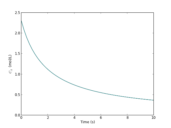
You can see the solution is near two seconds. Now we create an interpolating function to evaluate the solution. We will plot the interpolating function on a finer grid to make sure it seems reasonable.
ca_func = interp1d(tspan, Ca, 'cubic')

itime = np.linspace(0, 10, 200)

plt.figure()
plt.plot(tspan, Ca, '.')
plt.plot(itime, ca_func(itime), 'b-')

plt.xlabel('Time (s)')
plt.ylabel('$C_A$ (mol/L)')
plt.legend(['solution','interpolated'])
plt.savefig('images/ode-specific-2.png')
plt.show()
>>> >>> >>> <matplotlib.figure.Figure object at 0x1b2dfed0>
[<matplotlib.lines.Line2D object at 0x1c103b90>]
[<matplotlib.lines.Line2D object at 0x1c107050>]
>>> <matplotlib.text.Text object at 0x1c0e65d0>
<matplotlib.text.Text object at 0x1b95bfd0>
<matplotlib.legend.Legend object at 0x1c107550>
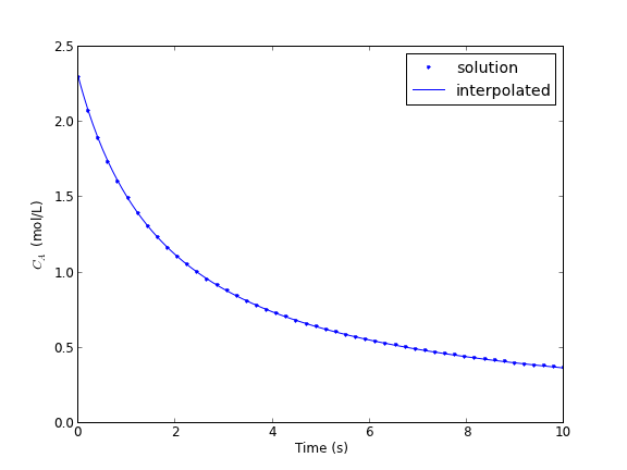
that loos pretty reasonable. Now we solve the problem.
tguess = 2.0
tsol, = fsolve(lambda t: 1.0 - ca_func(t), tguess)
print tsol

# you might prefer an explicit function
def func(t):
    return 1.0 - ca_func(t)

tsol2, = fsolve(func, tguess)
print tsol2
>>> 2.4574668235
>>> ... ... >>> 2.4574668235
That is it. Interpolation can provide a simple way to evaluate the numerical solution of an ODE at other values.
For completeness we examine a final way to construct the function. We can actually integrate the ODE in the function to evaluate the solution at the point of interest. If it is not computationally expensive to evaluate the ODE solution this works fine. Note, however, that the ODE will get integrated from 0 to the value t for each iteration of fsolve.
def func(t):
    tspan = [0, t]
    sol = odeint(dCadt, Ca0, tspan)
    return 1.0 - sol[-1]

tsol3, = fsolve(func, tguess)
print tsol3
... ... ... >>> >>> 2.45746688202
Copyright (C) 2013 by John Kitchin. See the License for information about copying.