Better interpolate than never

Posted February 02, 2013 at 09:00 AM | categories: interpolation | tags:

Updated February 27, 2013 at 02:42 PM

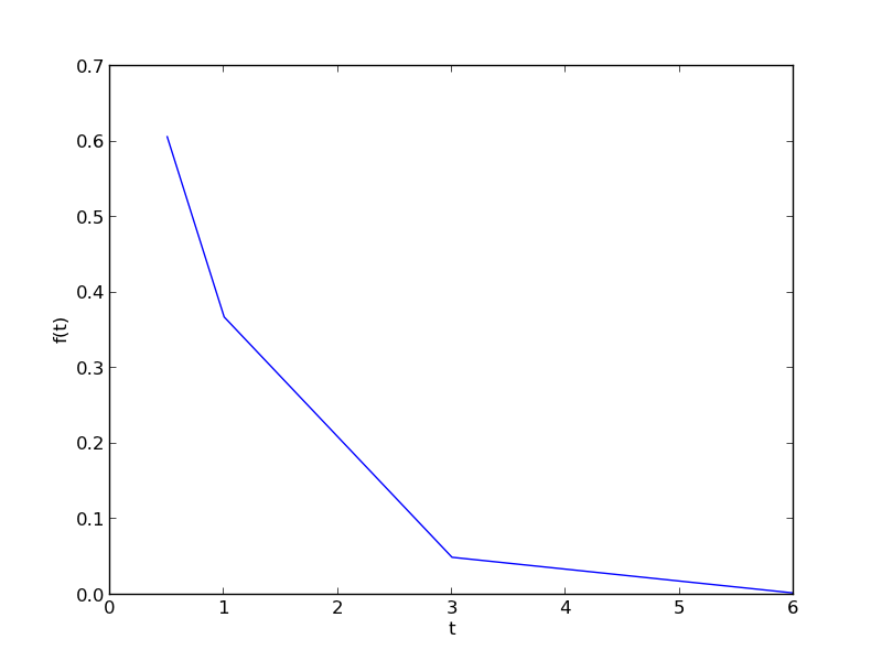
We often have some data that we have obtained in the lab, and we want to solve some problem using the data. For example, suppose we have this data that describes the value of f at time t.

import matplotlib.pyplot as plt

t = [0.5, 1, 3, 6]
f = [0.6065,    0.3679,    0.0498,    0.0025]
plt.plot(t,f)
plt.xlabel('t')
plt.ylabel('f(t)')
plt.savefig('images/interpolate-1.png')

>>> >>> >>> [<matplotlib.lines.Line2D object at 0x04D18730>]
<matplotlib.text.Text object at 0x04BEE8B0>
<matplotlib.text.Text object at 0x04C03970>

1 Estimate the value of f at t=2.

This is a simple interpolation problem.

from scipy.interpolate import interp1d

g = interp1d(t, f) # default is linear interpolation

print g(2)
print g([2, 3, 4])

>>> >>> >>> 0.20885
[ 0.20885     0.0498      0.03403333]

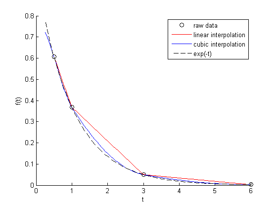
The function we sample above is actually f(t) = exp(-t). The linearly interpolated example is not too accurate.

import numpy as np
print np.exp(-2)

0.135335283237

2 improved interpolation?

we can tell interp1d to use a different interpolation scheme such as cubic polynomial splines like this. For nonlinear functions, this may improve the accuracy of the interpolation, as it implicitly includes information about the curvature by fitting a cubic polynomial over neighboring points.

g2 = interp1d(t, f, 'cubic')
print g2(2)
print g2([2, 3, 4])

0.108481818182
[ 0.10848182  0.0498      0.08428727]

Interestingly, this is a different value than Matlab's cubic interpolation. Let us show the cubic spline fit.

plt.figure()
plt.plot(t,f)
plt.xlabel('t')
plt.ylabel('f(t)')

x = np.linspace(0.5, 6)
fit = g2(x)
plt.plot(x, fit, label='fit')
plt.savefig('images/interpolation-2.png')

<matplotlib.figure.Figure object at 0x04EF2430>
[<matplotlib.lines.Line2D object at 0x04F20ED0>]
<matplotlib.text.Text object at 0x04EF2FF0>
<matplotlib.text.Text object at 0x04F060D0>
>>> >>> >>> [<matplotlib.lines.Line2D object at 0x04F17570>]

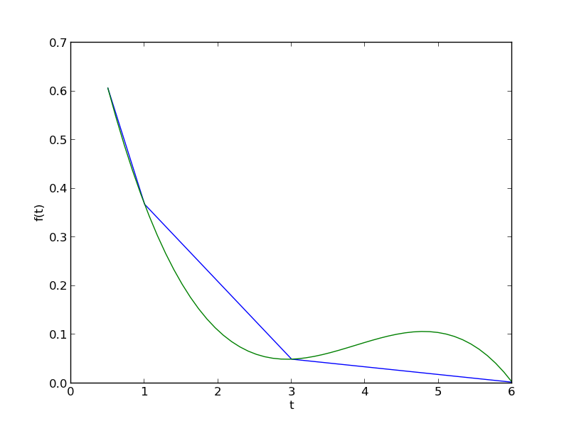
Wow. That is a weird looking fit. Very different from what Matlab produces. This is a good teaching moment not to rely blindly on interpolation! We will rely on the linear interpolation from here out which behaves predictably.

3 The inverse question

It is easy to interpolate a new value of f given a value of t. What if we want to know the time that f=0.2? We can approach this a few ways.

3.1 method 1

We setup a function that we can use fsolve on. The function will be equal to zero at the time. The second function will look like 0 = 0.2 - f(t). The answer for 0.2=exp(-t) is t = 1.6094. Since we use interpolation here, we will get an approximate answer.

from scipy.optimize import fsolve

def func(t):
    return 0.2 - g(t)

initial_guess = 2
ans, = fsolve(func, initial_guess)
print ans

>>> ... ... >>> >>> >>> 2.0556428796

3.2 method 2: switch the interpolation order

We can switch the order of the interpolation to solve this problem. An issue we have to address in this method is that the “x” values must be monotonically increasing. It is somewhat subtle to reverse a list in python. I will use the cryptic syntax of [::-1] instead of the list.reverse() function or reversed() function. list.reverse() actually reverses the list “in place”, which changes the contents of the variable. That is not what I want. reversed() returns an iterator which is also not what I want. [::-1] is a fancy indexing trick that returns a reversed list.

g3 = interp1d(f[::-1], t[::-1])

print g3(0.2)

>>> 2.0556428796

4 A harder problem

Suppose we want to know at what time is 1/f = 100? Now we have to decide what do we interpolate: f(t) or 1/f(t). Let us look at both ways and decide what is best. The answer to \(1/exp(-t) = 100\) is 4.6052

4.1 interpolate on f(t) then invert the interpolated number

def func(t):
    'objective function. we do some error bounds because we cannot interpolate out of the range.'
    if t < 0.5: t=0.5
    if t > 6: t = 6
    return 100 - 1.0 / g(t)   

initial_guess = 4.5
a1, = fsolve(func, initial_guess)
print a1
print 'The %error is {0:%}'.format((a1 - 4.6052)/4.6052)

... ... ... ... >>> >>> >>> 5.52431289641
The %error is 19.958154%

4.2 invert f(t) then interpolate on 1/f

ig = interp1d(t, 1.0 / np.array(f))

def ifunc(t):
    if t < 0.5: t=0.5
    if t > 6: t = 6
    return 100 - ig(t)   

initial_guess = 4.5
a2, = fsolve(ifunc, initial_guess)
print a2
print 'The %error is {0:%}'.format((a2 - 4.6052)/4.6052)

>>> ... ... ... ... >>> >>> >>> 3.6310782241
The %error is -21.152649%

5 Discussion

In this case you get different errors, one overestimates and one underestimates the answer, and by a lot: ± 20%. Let us look at what is happening.

import matplotlib.pyplot as plt
import numpy as np
from scipy.interpolate import interp1d

t = [0.5, 1, 3, 6]
f = [0.6065,    0.3679,    0.0498,    0.0025]

x = np.linspace(0.5, 6)


g = interp1d(t, f) # default is linear interpolation
ig = interp1d(t, 1.0 / np.array(f))

plt.figure()
plt.plot(t, 1 / np.array(f), 'ko ', label='data')
plt.plot(x, 1 / g(x), label='1/interpolated f(x)')
plt.plot(x, ig(x), label='interpolate on 1/f(x)')
plt.plot(x, 1 / np.exp(-x), 'k--', label='1/exp(-x)')
plt.xlabel('t')
plt.ylabel('1/f(t)')
plt.legend(loc='best')
plt.savefig('images/interpolation-3.png')

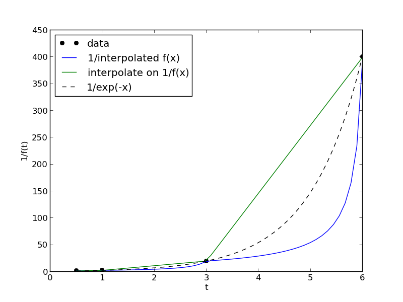
You can see that the 1/interpolated f(x) underestimates the value, while interpolated (1/f(x)) overestimates the value. This is an example of where you clearly need more data in that range to make good estimates. Neither interpolation method is doing a great job. The trouble in reality is that you often do not know the real function to do this analysis. Here you can say the time is probably between 3.6 and 5.5 where 1/f(t) = 100, but you can not read much more than that into it. If you need a more precise answer, you need better data, or you need to use an approach other than interpolation. For example, you could fit an exponential function to the data and use that to estimate values at other times.

So which is the best to interpolate? I think you should interpolate the quantity that is linear in the problem you want to solve, so in this case I think interpolating 1/f(x) is better. When you use an interpolated function in a nonlinear function, strange, unintuitive things can happen. That is why the blue curve looks odd. Between data points are linear segments in the original interpolation, but when you invert them, you cause the curvature to form.

org-mode source

The Kitchin Research Group

Chemical Engineering at Carnegie Mellon University