Estimating the boiling point of water
Posted February 04, 2013 at 09:00 AM | categories: uncategorized | tags: thermodynamics
Updated March 06, 2013 at 04:30 PM
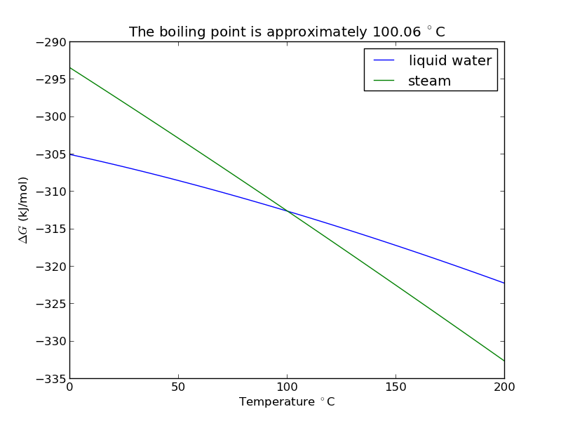
I got distracted looking for Shomate parameters for ethane today, and came across this website on predicting the boiling point of water using the Shomate equations. The basic idea is to find the temperature where the Gibbs energy of water as a vapor is equal to the Gibbs energy of the liquid.
import matplotlib.pyplot as plt
Liquid water (\url{http://webbook.nist.gov/cgi/cbook.cgi?ID=C7732185&Units=SI&Mask=2#Thermo-Condensed})
# valid over 298-500

Hf_liq = -285.830   # kJ/mol
S_liq = 0.06995     # kJ/mol/K
shomateL = [-203.6060,
            1523.290,
           -3196.413,
            2474.455,
               3.855326,
            -256.5478,
            -488.7163,
            -285.8304]
Gas phase water (\url{http://webbook.nist.gov/cgi/cbook.cgi?ID=C7732185&Units=SI&Mask=1&Type=JANAFG&Table=on#JANAFG})
Interestingly, these parameters are listed as valid only above 500K. That means we have to extrapolate the values down to 298K. That is risky for polynomial models, as they can deviate substantially outside the region they were fitted to.
Hf_gas = -241.826  # kJ/mol
S_gas = 0.188835   # kJ/mol/K

shomateG = [30.09200,
             6.832514,
             6.793435,
            -2.534480,
             0.082139,
          -250.8810,
           223.3967,
          -241.8264]
Now, we wan to compute G for each phase as a function of T
import numpy as np

T = np.linspace(0, 200) + 273.15
t = T / 1000.0

sTT = np.vstack([np.log(t),
                 t,
                 (t**2) / 2.0,
                 (t**3) / 3.0,
                 -1.0 / (2*t**2),
                 0 * t,
                 t**0,
                 0 * t**0]).T / 1000.0

hTT = np.vstack([t,
                 (t**2)/2.0,
                 (t**3)/3.0,
                 (t**4)/4.0,
                 -1.0 / t,
                 1 * t**0,
                 0 * t**0,
                 -1 * t**0]).T

Gliq = Hf_liq + np.dot(hTT, shomateL) - T*(np.dot(sTT, shomateL))
Ggas = Hf_gas + np.dot(hTT, shomateG) - T*(np.dot(sTT, shomateG))

from scipy.interpolate import interp1d
from scipy.optimize import fsolve

f = interp1d(T, Gliq - Ggas)
bp, = fsolve(f, 373)
print 'The boiling point is {0} K'.format(bp)
>>> >>> >>> >>> ... ... ... ... ... ... ... >>> >>> ... ... ... ... ... ... ... >>> >>> >>> >>> ... >>> >>> >>> >>> >>> The boiling point is 373.206081312 K
plt.figure(); plt.clf()
plt.plot(T-273.15, Gliq, T-273.15, Ggas)
plt.legend(['liquid water', 'steam'])

plt.xlabel('Temperature $^\circ$C')
plt.ylabel('$\Delta G$ (kJ/mol)')
plt.title('The boiling point is approximately {0:1.2f} $^\circ$C'.format(bp-273.15))
plt.savefig('images/boiling-water.png')
<matplotlib.figure.Figure object at 0x050D2E30>
[<matplotlib.lines.Line2D object at 0x051AB610>, <matplotlib.lines.Line2D object at 0x051B4C90>]
<matplotlib.legend.Legend object at 0x051B9030>
>>> <matplotlib.text.Text object at 0x0519E390>
<matplotlib.text.Text object at 0x050FB390>
<matplotlib.text.Text object at 0x050FBFB0>
1 Summary
The answer we get us 0.05 K too high, which is not bad considering we estimated it using parameters that were fitted to thermodynamic data and that had finite precision and extrapolated the steam properties below the region the parameters were stated to be valid for.
Copyright (C) 2013 by John Kitchin. See the License for information about copying.