The Kitchin Research Group

Matlab post

The idea here is to formulate a set of linear equations that is easy to solve. We can express the equations in terms of our unknown fitting parameters \(p_i\) as:

x1^0*p0 + x1*p1 = y1
x2^0*p0 + x2*p1 = y2
x3^0*p0 + x3*p1 = y3
etc...

Which we write in matrix form as \(A p = y\) where \(A\) is a matrix of column vectors, e.g. [1, x_i]. \(A\) is not a square matrix, so we cannot solve it as written. Instead, we form \(A^T A p = A^T y\) and solve that set of equations.

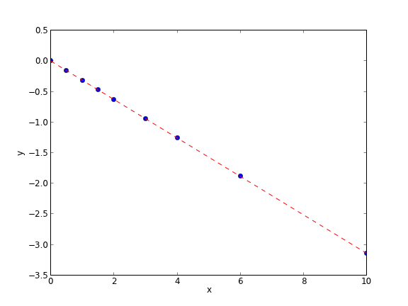
import numpy as np
x = np.array([0, 0.5, 1, 1.5, 2.0, 3.0, 4.0, 6.0, 10])
y = np.array([0, -0.157, -0.315, -0.472, -0.629, -0.942, -1.255, -1.884, -3.147])

A = np.column_stack([x**0, x])

M = np.dot(A.T, A)
b = np.dot(A.T, y)

i1, slope1 = np.dot(np.linalg.inv(M), b)
i2, slope2 = np.linalg.solve(M, b) # an alternative approach.

print i1, slope1
print i2, slope2

# plot data and fit
import matplotlib.pyplot as plt

plt.plot(x, y, 'bo')
plt.plot(x, np.dot(A, [i1, slope1]), 'r--')
plt.xlabel('x')
plt.ylabel('y')
plt.savefig('images/la-line-fit.png')

0.00062457337884 -0.3145221843
0.00062457337884 -0.3145221843

This method can be readily extended to fitting any polynomial model, or other linear model that is fit in a least squares sense. This method does not provide confidence intervals.

Copyright (C) 2013 by John Kitchin. See the License for information about copying.

org-mode source