Linear regression with confidence intervals.
Posted February 18, 2013 at 09:00 AM | categories: confidence interval, data analysis, linear regression | tags:
Updated February 27, 2013 at 02:39 PM
Matlab post Fit a fourth order polynomial to this data and determine the confidence interval for each parameter. Data from example 5-1 in Fogler, Elements of Chemical Reaction Engineering.
We want the equation \(Ca(t) = b0 + b1*t + b2*t^2 + b3*t^3 + b4*t^4\) fit to the data in the least squares sense. We can write this in a linear algebra form as: T*p = Ca where T is a matrix of columns [1 t t^2 t^3 t^4], and p is a column vector of the fitting parameters. We want to solve for the p vector and estimate the confidence intervals.
import numpy as np
from scipy.stats.distributions import  t

time = np.array([0.0, 50.0, 100.0, 150.0, 200.0, 250.0, 300.0])
Ca = np.array([50.0, 38.0, 30.6, 25.6, 22.2, 19.5, 17.4])*1e-3

T = np.column_stack([time**0, time, time**2, time**3, time**4])

p, res, rank, s = np.linalg.lstsq(T, Ca)
# the parameters are now in p

# compute the confidence intervals
n = len(Ca)
k = len(p)

sigma2 = np.sum((Ca - np.dot(T, p))**2) / (n - k)  # RMSE

C = sigma2 * np.linalg.inv(np.dot(T.T, T)) # covariance matrix
se = np.sqrt(np.diag(C)) # standard error

alpha = 0.05 # 100*(1 - alpha) confidence level

sT = t.ppf(1.0 - alpha/2.0, n - k) # student T multiplier
CI = sT * se

for beta, ci in zip(p, CI):
    print '{2: 1.2e} [{0: 1.4e} {1: 1.4e}]'.format(beta - ci, beta + ci, beta)

SS_tot = np.sum((Ca - np.mean(Ca))**2)
SS_err = np.sum((np.dot(T, p) - Ca)**2)

#  http://en.wikipedia.org/wiki/Coefficient_of_determination
Rsq = 1 - SS_err/SS_tot
print 'R^2 = {0}'.format(Rsq)

# plot fit
import matplotlib.pyplot as plt
plt.plot(time, Ca, 'bo', label='raw data')
plt.plot(time, np.dot(T, p), 'r-', label='fit')
plt.xlabel('Time')
plt.ylabel('Ca (mol/L)')
plt.legend(loc='best')
plt.savefig('images/linregress-conf.png')
 5.00e-02 [ 4.9680e-02  5.0300e-02]
-2.98e-04 [-3.1546e-04 -2.8023e-04]
 1.34e-06 [ 1.0715e-06  1.6155e-06]
-3.48e-09 [-4.9032e-09 -2.0665e-09]
 3.70e-12 [ 1.3501e-12  6.0439e-12]
R^2 = 0.999986967246
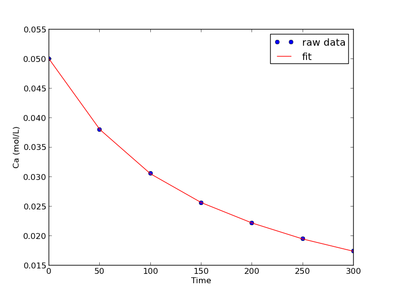
A fourth order polynomial fits the data well, with a good R^2 value. All of the parameters appear to be significant, i.e. zero is not included in any of the parameter confidence intervals. This does not mean this is the best model for the data, just that the model fits well.
Copyright (C) 2013 by John Kitchin. See the License for information about copying.