Modeling a transient plug flow reactor
Posted March 06, 2013 at 03:51 PM | categories: animation, pde | tags: reaction engineering
Updated March 25, 2013 at 09:50 AM
The PDE that describes the transient behavior of a plug flow reactor with constant volumetric flow rate is:
\( \frac{\partial C_A}{\partial dt} = -\nu_0 \frac{\partial C_A}{\partial dV} + r_A \).
To solve this numerically in python, we will utilize the method of lines. The idea is to discretize the reactor in volume, and approximate the spatial derivatives by finite differences. Then we will have a set of coupled ordinary differential equations that can be solved in the usual way. Let us simplify the notation with \(C = C_A\), and let \(r_A = -k C^2\). Graphically this looks like this:

This leads to the following set of equations:
\begin{eqnarray} \frac{dC_0}{dt} &=& 0 \text{ (entrance concentration never changes)} \\ \frac{dC_1}{dt} &=& -\nu_0 \frac{C_1 - C_0}{V_1 - V_0} - k C_1^2 \\ \frac{dC_2}{dt} &=& -\nu_0 \frac{C_2 - C_1}{V_2 - V_1} - k C_2^2 \\ \vdots \\ \frac{dC_4}{dt} &=& -\nu_0 \frac{C_4 - C_3}{V_4 - V_3} - k C_4^2 \end{eqnarray}Last, we need initial conditions for all the nodes in the discretization. Let us assume the reactor was full of empty solvent, so that \(C_i = 0\) at \(t=0\). In the next block of code, we get the transient solutions, and the steady state solution.
import numpy as np
from scipy.integrate import odeint

Ca0 = 2     # Entering concentration
vo = 2      # volumetric flow rate
volume = 20 # total volume of reactor, spacetime = 10
k = 1       # reaction rate constant

N = 100     # number of points to discretize the reactor volume on

init = np.zeros(N)    # Concentration in reactor at t = 0
init[0] = Ca0         # concentration at entrance

V = np.linspace(0, volume, N) # discretized volume elements
tspan = np.linspace(0, 25)    # time span to integrate over

def method_of_lines(C, t):
    'coupled ODES at each node point'
    D = -vo * np.diff(C) / np.diff(V) - k * C[1:]**2
    return np.concatenate([[0], #C0 is constant at entrance
                            D])


sol = odeint(method_of_lines, init, tspan)

# steady state solution
def pfr(C, V):
    return 1.0 / vo * (-k * C**2)

ssol = odeint(pfr, Ca0, V)
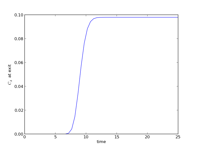
The transient solution contains the time dependent behavior of each node in the discretized reactor. Each row contains the concentration as a function of volume at a specific time point. For example, we can plot the concentration of A at the exit vs. time (that is, the last entry of each row) as:
import matplotlib.pyplot as plt
plt.plot(tspan, sol[:, -1])
plt.xlabel('time')
plt.ylabel('$C_A$ at exit')
plt.savefig('images/transient-pfr-1.png')
[<matplotlib.lines.Line2D object at 0x05A18830>]
<matplotlib.text.Text object at 0x059FE1D0>
<matplotlib.text.Text object at 0x05A05270>

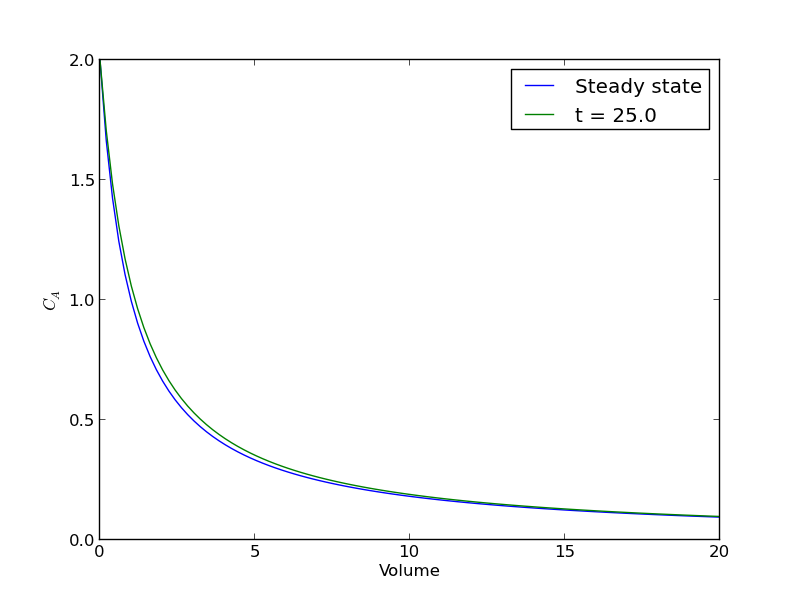
After approximately one space time, the steady state solution is reached at the exit. For completeness, we also examine the steady state solution.
plt.figure()
plt.plot(V, ssol, label='Steady state')
plt.plot(V, sol[-1], label='t = {}'.format(tspan[-1]))
plt.xlabel('Volume')
plt.ylabel('$C_A$')
plt.legend(loc='best')
plt.savefig('images/transient-pfr-2.png')

There is some minor disagreement between the final transient solution and the steady state solution. That is due to the approximation in discretizing the reactor volume. In this example we used 100 nodes. You get better agreement with a larger number of nodes, say 200 or more. Of course, it takes slightly longer to compute then, since the number of coupled odes is equal to the number of nodes.
We can also create an animated gif to show how the concentration of A throughout the reactor varies with time. Note, I had to install ffmpeg (http://ffmpeg.org/) to save the animation.
from matplotlib import animation

# make empty figure
fig = plt.figure()
ax = plt.axes(xlim=(0, 20), ylim=(0, 2))
line, = ax.plot(V, init, lw=2)

def animate(i):
    line.set_xdata(V)
    line.set_ydata(sol[i])
    ax.set_title('t = {0}'.format(tspan[i]))
    ax.figure.canvas.draw()
    return line,


anim = animation.FuncAnimation(fig, animate, frames=50,  blit=True)

anim.save('images/transient_pfr.mp4', fps=10)
http://jkitchin.github.com/media/transient_pfr.mp4
You can see from the animation that after about 10 time units, the solution is not changing further, suggesting steady state has been reached.
Copyright (C) 2013 by John Kitchin. See the License for information about copying.