Neural networks for regression with autograd
Posted November 18, 2017 at 02:20 PM | categories: python, autograd | tags:
Today we are going to take a meandering path to using autograd to train a neural network for regression. First let's consider this very general looking nonlinear model that we might fit to data. There are 10 parameters in it, so we should expect we can get it to fit some data pretty well.
\(y = b1 + w10 tanh(w00 x + b00) + w11 tanh(w01 x + b01) + w12 tanh(w02 x + b02)\)
We will use it to fit data that is generated from \(y = x^\frac{1}{3}\). First, we just do a least_squares fit. This function can take a jacobian function, so we provide one using autograd.
import autograd.numpy as np
from autograd import jacobian

from scipy.optimize import curve_fit

# Some generated data
X = np.linspace(0, 1)
Y = X**(1. / 3.)

def model(x, *pars):
    b1, w10, w00, b00, w11, w01, b01, w12, w02, b02 = pars
    pred = b1 + w10 * np.tanh(w00 * x + b00) + w11 * np.tanh(w01 * x + b01) + w12 * np.tanh(w02 * x + b02)
    return pred


def resid(pars):
    return Y - model(X, *pars)
MSE: 0.0744600049689
We will look at some timing of this regression. Here we do not provide a jacobian.
%%timeit
pars = least_squares(resid, np.random.randn(10)*0.1).x
1.21 s ± 42.7 ms per loop (mean ± std. dev. of 7 runs, 1 loop each)
And here we do provide one. It takes a lot longer to do this. We do have a jacobian of 10 parameters, so that ends up being a lot of extra computations to do.
%%timeit
pars = least_squares(resid, np.random.randn(10)*0.1, jac=jacobian(resid)).x
24.1 s ± 1.61 s per loop (mean ± std. dev. of 7 runs, 1 loop each)
We will print these parameters for reference later.
b1, w10, w00, b00, w11, w01, b01, w12, w02, b02 = pars

print([w00, w01, w02], [b00, b01, b02])
print([w10, w11, w12], b1)
[5.3312122926210703, 54.6923797622945, -0.50881373227993232] [2.9834159679095662, 2.6062295455987199, -2.3782572250527778]
[42.377172168160477, 22.036104340171004, -50.075636975961089] -113.179935862
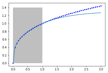
Let's just make sure the fit looks ok. I am going to plot it outside the fitted region to see how it extrapolates. The shaded area shows the region we did the fitting in.
X2 = np.linspace(0, 3)
Y2 = X2**(1. / 3.)

Z2 = model(X2, *pars)

plt.plot(X2, Y2, 'b.', label='analytical')
plt.plot(X2, Z2, label='model')
plt.fill_between(X2 < 1, 0, 1.4, facecolor='gray', alpha=0.5)

You can seen it fits pretty well from 0 to 1 where we fitted it, but outside that the model is not accurate. Our model is not that related to the true function of the model, so there is no reason to expect it should extrapolate.
I didn't pull that model out of nowhere. Let's rewrite it in a few steps. If we think of tanh as a function that operates element-wise on a vector, we could write that equation more compactly at:
                              [w00 * x + b01]
y = [w10, w11, w12] @ np.tanh([w01 * x + b01]) + b1
                              [w02 * x + b02]
We can rewrite this one more time in matrix notation:
y = w1 @ np.tanh(w0 @ x + b0) + b1
Another way to read these equations is that we have an input of x. We multiply the input by a vector weights (w0), add a vector of offsets (biases), b0, activate that by the nonlinear tanh function, then multiply that by a new set of weights, and add a final bias. We typically call this kind of model a neural network. There is an input layer, one hidden layer with 3 neurons that are activated by tanh, and one output layer with linear activation.
Autograd was designed in part for building neural networks. In the next part of this post, we reformulate this regression as a neural network. This code is lightly adapted from https://github.com/HIPS/autograd/blob/master/examples/neural_net_regression.py.
The first function initializes the weights and biases for each layer in our network. It is standard practice to initialize them to small random numbers to avoid any unintentional symmetries that might occur from a systematic initialization (e.g. all ones or zeros). The second function sets up the neural network and computes its output.
from autograd import grad
import autograd.numpy.random as npr
from autograd.misc.optimizers import adam

def init_random_params(scale, layer_sizes, rs=npr.RandomState(0)):
    """Build a list of (weights, biases) tuples, one for each layer."""
    return [(rs.randn(insize, outsize) * scale,   # weight matrix
             rs.randn(outsize) * scale)           # bias vector
            for insize, outsize in zip(layer_sizes[:-1], layer_sizes[1:])]

def nn_predict(params, inputs, activation=np.tanh):
    for W, b in params[:-1]:
        outputs = np.dot(inputs, W) + b
        inputs = activation(outputs)
    # no activation on the last layer
    W, b = params[-1]
    return np.dot(inputs, W) + b
Here we use the first function to define the weights and biases for a neural network with one input, one hidden layer of 3 neurons, and one output layer.
init_scale = 0.1

# Here is our initial guess:
params = init_random_params(init_scale, layer_sizes=[1, 3, 1])
for i, wb in enumerate(params):
    W, b = wb
    print('w{0}: {1}, b{0}: {2}'.format(i, W.shape, b.shape))
w0: (1, 3), b0: (3,)
w1: (3, 1), b1: (1,)
You can see w0 is a column vector of weights, and there are three biases in b0. W1 in contrast, is a row vector of weights, with one bias. So 10 parameters in total, like we had before. We will create an objective function of the mean squared error again, and a callback function to show us the progress.
Then we run the optimization step iteratively until we get our objective function below a tolerance we define.
def objective(params, _):
    pred = nn_predict(params, X.reshape([-1, 1]))
    err = Y.reshape([-1, 1]) - pred
    return np.mean(err**2)


def callback(params, step, g):
    if step % 250 == 0:
        print("Iteration {0:3d} objective {1:1.2e}".format(i * N + step,
                                                           objective(params, step)))

N = 500
NMAX = 20

for i in range(NMAX):
    params = adam(grad(objective), params,
                  step_size=0.01, num_iters=N, callback=callback)
    if objective(params, _) < 2e-5:
        break
Iteration   0 objective 5.30e-01
Iteration 250 objective 4.52e-03
Iteration 500 objective 4.17e-03
Iteration 750 objective 1.86e-03
Iteration 1000 objective 1.63e-03
Iteration 1250 objective 1.02e-03
Iteration 1500 objective 6.30e-04
Iteration 1750 objective 4.54e-04
Iteration 2000 objective 3.25e-04
Iteration 2250 objective 2.34e-04
Iteration 2500 objective 1.77e-04
Iteration 2750 objective 1.35e-04
Iteration 3000 objective 1.04e-04
Iteration 3250 objective 7.86e-05
Iteration 3500 objective 5.83e-05
Iteration 3750 objective 4.46e-05
Iteration 4000 objective 3.39e-05
Iteration 4250 objective 2.66e-05
Iteration 4500 objective 2.11e-05
Iteration 4750 objective 1.71e-05
Let's compare these parameters to the previous ones we got.
for i, wb in enumerate(params):
    W, b = wb
    print('w{0}: {1}, b{0}: {2}'.format(i, W, b))
w0: [[ -0.71332351   3.23209728 -32.51135373]], b0: [ 0.45819205  0.19314303 -0.8687    ]
w1: [[-0.53699549]
 [ 0.39522207]
 [-1.05457035]], b1: [-0.58005452]
These look pretty different. It is not too surprising that there could be more than one set of these parameters that give similar fits. The original data only requires two parameters to create it: \(y = a x^b\), where \(x=1\) and \(b=1/3\). We have 8 extra parameters of flexibility in this model.
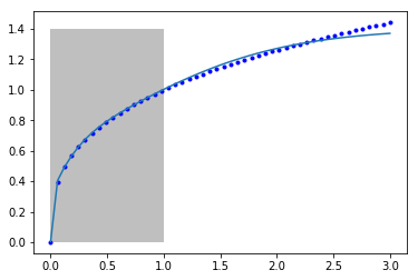
Let's again examine the fit of our model to the data.
Z2 = nn_predict(params, X2.reshape([-1, 1]))

plt.plot(X2, Y2, 'b.', label='analytical')
plt.plot(X2, Z2, label='NN')
plt.fill_between(X2 < 1, 0, 1.4, facecolor='gray', alpha=0.5)

Once again, we can see that between 0 and 1 where the model was fitted we get a good fit, but past that the model does not fit the known function well. It is coincidentally better than our previous model, but as before it is not advisable to use this model for extrapolation. Even though we say it "learned" something about the data, it clearly did not learn the function \(y=x^{1/3}\). It did "learn" some approximation to it in the region of x=0 to 1. Of course, it did not learn anything that the first nonlinear regression model didn't learn.
Now you know the secret of a neural network, it is just a nonlinear model. Without the activation, it is just a linear model. So, why use linear regression, when you can use an unactivated neural network and call it AI?
Copyright (C) 2017 by John Kitchin. See the License for information about copying.
Org-mode version = 9.1.2