Sensitivity analysis with odeint and autograd
Posted September 13, 2019 at 09:56 AM | categories: ode, autograd | tags:
In this previous post I showed a way to do sensitivity analysis of the solution of a differential equation to parameters in the equation using autograd. The basic approach was to write a differentiable integrator, and then use it in a function so that autograd could take the derivative.
Since that time, autograd has added derivative support for scipy.integrate.odeint. In this post we examine that. As usual with autograd, we have to import the autograd version of numpy, and the autograd version of odeint. We will find the derivative of the solution to an ODE (which is an array) so we need to also import the jacobian function. Finally, there is a subtle, and non-obvious requirement that we need to import the autograd tuple. That ensures that the variables are differentiable through the tuple we will use for the arguments.
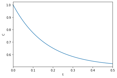
The differential equation we solve returns the concentration of a species as a function of time, and the solution depends on two parameters, i.e. \(C = f(t; k_1, k_{-1})\), and we are interested in the time-dependent sensitivity of \(C\) with respect to those parameters. The approach we use is to define a function that has those parameters as arguments. The function will solve the ODE and return the time-dependent solution. First we make that solution, mostly to see that the autograd version of odeint works.
import autograd.numpy as np
from autograd.scipy.integrate import odeint
from autograd import jacobian
from autograd.builtins import tuple

import matplotlib.pyplot as plt

Ca0 = 1.0
k1 = k_1 = 3.0

tspan = np.linspace(0, 0.5)

def C(K):
    k1, k_1 = K
    def dCdt(Ca, t, k1, k_1):
        return -k1 * Ca + k_1 * (Ca0 - Ca)
    sol = odeint(dCdt, Ca0, tspan, tuple((k1, k_1)))
    return sol

plt.plot(tspan, C([k1, k_1]))
plt.xlim([tspan.min(), tspan.max()])
plt.xlabel('t')
plt.ylabel('C');
<Figure size 432x288 with 1 Axes>
Now, the solution is an array, and we want the derivative of C with respect to the parameters at each time point. That means we want the jacobian derivative of the output with respect to the input. Here is the autograd approach to doing that. The jacobian function returns a function that we can evaluate to get the derivatives.
import time
t0 = time.time()
dCdk = jacobian(C, 0)


k_sensitivity = dCdk(np.array([k1, k_1]))

k1_sensitivity = k_sensitivity[:, 0, 0]
k_1_sensitivity = k_sensitivity[:, 0, 1]

plt.plot(tspan, np.abs(k1_sensitivity), label='dC/dk1')
plt.plot(tspan, np.abs(k_1_sensitivity), label='dC/dk_1')
plt.legend(loc='best')
plt.xlabel('t')
plt.ylabel('sensitivity')
print(f'Elapsed time = {time.time() - t0:1.1f} seconds')
Elapsed time = 38.2 seconds
<Figure size 432x288 with 1 Axes>
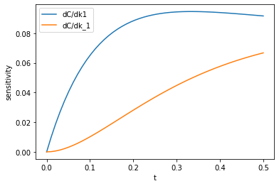
That looks similar to the results from before. It is pretty slow I think, that took more than half a minute to work out. That is still faster and probably more correct than if I had to do it by hand. In contrast, however, the finite difference code below is comparatively very fast! I don't know what is slow in the autograd implementation. I guess it is an implementation detail.
import numdifftools as nd
t0 = time.time()

fdk1, fdk_1 = nd.Jacobian(C)([k1, k_1]).T
print(f'Elapsed time = {time.time() - t0:1.1f} seconds')

plt.plot(tspan, np.abs(fdk1), label='fd dC/dk1')
plt.plot(tspan, np.abs(fdk_1), label='fd dC/dk_1')
plt.plot(tspan, np.abs(k1_sensitivity), 'y--', label='dC/dk1')
plt.plot(tspan, np.abs(k_1_sensitivity),'m--', label='dC/dk_1')
plt.legend(loc='best');
plt.xlabel('t');
plt.ylabel('sensitivity');
Elapsed time = 0.1 seconds
<Figure size 432x288 with 1 Axes>
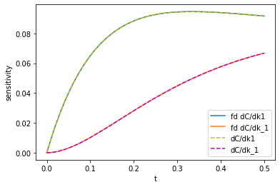
You can see the two results are visually indistinguishable. Even the code is pretty similar. I would tend to prefer the autograd way since it should be less sensitive to finite difference artifacts, but it is nice to have an independent way to test if it is working.
Copyright (C) 2019 by John Kitchin. See the License for information about copying.
Org-mode version = 9.2.3