Kolmogorov-Arnold Networks (KANs) and Lennard Jones

| categories: uncategorized | tags:

KANs have been a hot topic of discussion recently (https://arxiv.org/abs/2404.19756). Here I explore using them as an alternative to a neural network for a simple atomistic potential using Lennard Jones data. I adapted this code from https://github.com/KindXiaoming/pykan/blob/master/hellokan.ipynb.

TL;DR It was easy to make the model, and it fit this simple data very well. It does not extrapolate in this example, and it is not obvious what the extrapolation behavior should be.

1. Create a dataset

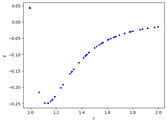
We leverage the create_dataset function to generate the dataset here. I chose a range with some modest nonlinearity, and the minimum.

import matplotlib.pyplot as plt
import torch
from kan import create_dataset, KAN

def LJ(r):
    r6 = r**6
    return 1 / r6**2 - 1 / r6

dataset = create_dataset(LJ, n_var=1, ranges=[0.95, 2.0],
                         train_num=50)

plt.plot(dataset['train_input'], dataset['train_label'], 'b.')
plt.xlabel('r')
plt.ylabel('E');

2. Create and train the model

We start by making the model. We are going to model a Lennard-Jones potential with one input, the distance between two atoms, and one output. We start with a width of 2 "neurons".

model = KAN(width=[1, 2, 1])

Training is easy. You can even run this cell several times.

model.train(dataset, opt="LBFGS", steps=20);

model.plot()
train loss: 1.64e-04 | test loss: 1.46e-02 | reg: 6.72e+00 : 100%|██| 20/20 [00:03<00:00,  5.61it/s]

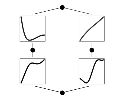
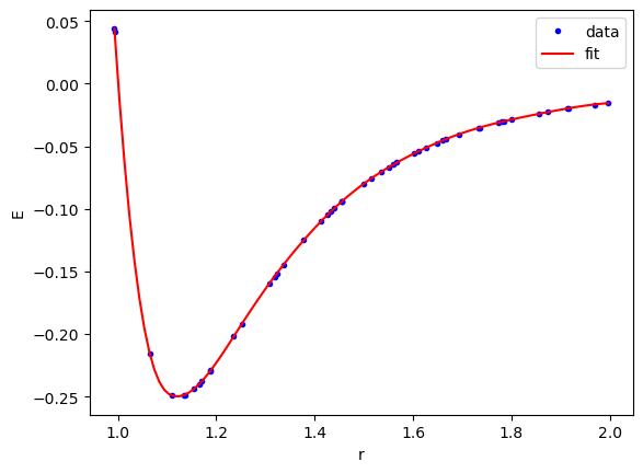
We can see here that the fit looks very good.

X = torch.linspace(dataset['train_input'].min(),
                   dataset['train_input'].max(), 100)[:, None]

plt.plot(dataset['train_input'], dataset['train_label'], 'b.', label='data')

plt.plot(X, model(X).detach().numpy(), 'r-', label='fit')
plt.legend()
plt.xlabel('r')
plt.ylabel('E');

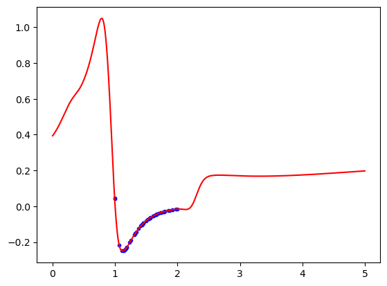
KANs do not save us from extrapolation issues though. I think a downside of KANs is it is not obvious what extrapolation behavior to expect. I guess it could be related to what happens in the spline representation of the functions. Eventually those have to extrapolate too.

X = torch.linspace(0, 5, 1000)[:, None]
plt.plot(dataset['train_input'], dataset['train_label'], 'b.')
plt.plot(X, model(X).detach().numpy(), 'r-');

It is early days for KANs, so many things we know about MLPs are still unknown for KANs. For example, with MLPs we know they extrapolate like the activation functions. Probably there is some insight like that to be had here, but it needs to be uncovered. With MLPs there are a lot of ways to regularize them for desired behavior. Probably that is true here too, and will be discovered. Similarly, there are many ways people have approached uncertainty quantification in MLPs that probably have some analog in KANs. Still, the ease of use suggests it could be promising for some applications.

Copyright (C) 2024 by John Kitchin. See the License for information about copying.

org-mode source

Org-mode version = 9.7-pre

Discuss on Twitter

A little more than a decade of the Kitchingroup blog

| categories: uncategorized | tags:

There are a few early entries I backdated, but this blog got started in its present form in January 2013. This entry marks entry #594. I started this blog as part of an exercise in switching from Matlab to Python, and the first hundred entries or so are just me solving a problem in Python that I had previously solved in Matlab. It then expanded to include lots of entries on Emacs and org-mode, and other research related topics from my group. Many entries simply document something I spent time working out and that I wanted to be able to find by Google later.

When I set the blog up, I enabled Google Analytics to see if anyone would look at. Recently Google announced they are shutting down the version of analytics I was using, and transitioning to a newer approach. They no longer collect data with the version this blog is using (since Oct last year), and they will delete the data this summer, so today I downloaded some of it to see what has happened over the past decade.

Anecdotally many people from around the world have told me how useful the blog was for them. Now, I have data to see how many people have been impacted by this blog. This figure shows that a lot of people spent time in some part of the blog over the past decade! The data suggests over 1M people viewed these pages over 2M times.

The peak usage was around 2020, and it has been trailing off since then. I have not been as active in posting since then. You can also see there is a very long build up to that peak.

The user group for the blog is truly world wide, including almost every country in this map. That is amazing!

Finally, I found the pages that were most viewed. It is interesting most of them are the older pages, and all about Python. I guess that means I should write more posts on Python.

I don't know what the future of the blog is. It is in need of an overhaul. The packages that build it still work, but are not actively maintained. I have also spent more time writing with Jupyter Book lately than the way I wrote this blog. It isn't likely to disappear any time soon, it sits rent-free in GitHUB pages.

To conclude, to everyone who has read these pages, thank you! It has been a lot of work to put together over the years, and I am glad to see many people have taken a look at it.

Copyright (C) 2024 by John Kitchin. See the License for information about copying.

org-mode source

Org-mode version = 9.7-pre

Discuss on Twitter

pycse YouTube Channel

| categories: uncategorized | tags:

Over the past few months, I have been making a series of short Python videos on YouTube. You can find the playlist at https://www.youtube.com/playlist?list=PL0sMmOaE_gs2yzwy54kLZk5c1ZH-Nh-62. They are not particularly well organized there, since I make them in the order I feel like, and when I have some spare time, so today I took some time to organize them by some topics here. If you find them useful, please subscribe to the channel and tell your friends about them!

Copyright (C) 2021 by John Kitchin. See the License for information about copying.

org-mode source

Org-mode version = 9.5

Discuss on Twitter

Integration of the heat capacity

| categories: uncategorized | tags:

From thermodynamics, the heat capacity is defined as \(C_p = \left(\frac{dH}{dT}\right)_P\). That means we can calculate the heat required to change the temperature of some material from the following integral:

\(H_2 - H_1 = Q = \int_{T_1}^{T_2} C_p(T) dT\)

In the range of 298-1200K, the heat capacity of CO2 is given by a Shomate polynomial:

\(C_p(t) = A + B t + C t^2 + D t^3 + E/t^2\) with units of J/mol/K.

where \(t = T / 1000\), and \(T\) is the temperature in K. The constants in the equation are

  value
A 24.99735
B 55.18696
C -33.69137
D 7.948387
E -0.136638
F -403.6075
G 228.2431
H -393.5224

1 Integrate the heat capacity

Use this information to compute the energy (Q in kJ/mol) required to raise the temperature of CO2 from 300K to 600K. You should use scipy.integrate.quad to perform the integration.


1.1 solution   solution

A =  24.99735
B =  55.18696
C = -33.69137
D =  7.948387
E = -0.136638
F = -403.6075
G =  228.2431
H = -393.5224

def Cp(T):
    t = T / 1000
    return A + B*t + C*t**2 + D*t**3 + E / t**2

from scipy.integrate import quad

dH, _ = quad(Cp, 300, 600)
print(f'The change in enthalpy is {dH / 1000:1.3f} kJ/mol')
The change in enthalpy is 12.841 kJ/mol


2 Verify via Δ H

The change in enthalpy (in kJ / mol) from standard state is

\(dH − dH_{298.15}= A t + B t^2/2 + C t^3/3 + D t^4/4 − E/t + F − H\)

again, \(t = T / 1000\).

Use this equation to compute the change in enthalpy when you increase the temperature from 300 K to 600 K.


2.1 solution   solution

def dH(T):
    t = T / 1000
    return A * t + B*t**2 / 2 + C * t**3 / 3 + D * t**4 / 4 - E/t + F - H

print(f'The change in enthalpy is {dH(600) - dH(300):1.3f} kJ/mol')
The change in enthalpy is 12.841 kJ/mol


Copyright (C) 2018 by John Kitchin. See the License for information about copying.

org-mode source

Org-mode version = 9.1.13

Discuss on Twitter

helm actions when there is no match

| categories: uncategorized | tags:

Sometimes you run out of matches in a helm selection buffer, and all that is left is the pattern you have typed in. It turns out you can perform some action on that pattern! Why would you do that? Suppose you are searching your bibliography, and you do not find what you are looking for. Then, you may want to send the pattern to Google, or some other search engine to see what comes up.

The key to handling this situation is to use two sources in your helm session. One that works on the candidates and deals with actions on them, and one that has no candidates, and works on the pattern. The variable helm-pattern contains what you typed in. We call the second source the Fallback option. The second source has no candidates, and we use (dummy) in place of the candidates.

It easy to add two sources. Here we define the sources as variables, and use the variables in the :sources list to the helm command.

(defun some-action (arg)
  (message-box "%s\n%s"
    (helm-get-selection)
    (helm-marked-candidates)))

(defun default-action (candidate)
  (browse-url
   (format
    "http://www.google.com/search?q=%s" (url-hexify-string helm-pattern))))

(defvar source1 '((name . "HELM")
                  (candidates . (1 2 3 4))
                  (action . (("open" . some-action)))))

(defvar fallback-source '((name . "fallback")
                          (dummy)
                          (action . (("Google" . default-action)))))

(helm :sources '(source1 fallback-source))
#<process open http://www.google.com/search?q=addtion%20pul>

When you run this, if you run out of search candidates, all that will be left is the fallback option, and when you press enter, it will launch a browser pointing to the google search for your pattern.

Copyright (C) 2015 by John Kitchin. See the License for information about copying.

org-mode source

Org-mode version = 8.2.10

Discuss on Twitter
Next Page »